Skewed generalized t distribution

In probability and statistics, the skewed generalized "t" distribution is a family of continuous probability distributions. The distribution was first introduced by Panayiotis Theodossiou^[1] in 1998. The distribution has since been used in different applications.^{[2][3][4][5][6][7]} There are different parameterizations for the skewed generalized t distribution.^[1][5]

${\displaystyle f_{\text{SGT}}(x;\mu ,\sigma ,\lambda ,p,q)={\frac {p}{2v\sigma q^{\frac {1}{p}}B({\frac {1}{p}},q)\left[1+{\frac {|x-\mu +m|^{p}}{q(v\sigma )^{p}(1+\lambda \operatorname {sgn}(x-\mu +m))^{p}}}\right]^{{\frac {1}{p}}+q}}}}$

where ${\displaystyle B}$ is the beta function, ${\displaystyle \mu }$ is the location parameter, ${\displaystyle \sigma >0}$ is the scale parameter, ${\displaystyle -1<\lambda <1}$ is the skewness parameter, and ${\displaystyle p>0}$ and ${\displaystyle q>0}$ are the parameters that control the kurtosis. ${\displaystyle m}$ and ${\displaystyle v}$ are not parameters, but functions of the other parameters that are used here to scale or shift the distribution appropriately to match the various parameterizations of this distribution.

In the original parameterization^[1] of the skewed generalized t distribution,

${\displaystyle m=\lambda v\sigma {\frac {2q^{\frac {1}{p}}B({\frac {2}{p}},q-{\frac {1}{p}})}{B({\frac {1}{p}},q)}}}$

and

${\displaystyle v={\frac {q^{-{\frac {1}{p}}}}{\sqrt {(1+3\lambda ^{2}){\frac {B({\frac {3}{p}},q-{\frac {2}{p}})}{B({\frac {1}{p}},q)}}-4\lambda ^{2}{\frac {B({\frac {2}{p}},q-{\frac {1}{p}})^{2}}{B({\frac {1}{p}},q)^{2}}}}}}}$.

These values for ${\displaystyle m}$ and ${\displaystyle v}$ yield a distribution with mean of ${\displaystyle \mu }$ if ${\displaystyle pq>1}$ and a variance of ${\displaystyle \sigma ^{2}}$ if ${\displaystyle pq>2}$. In order for ${\displaystyle m}$ to take on this value however, it must be the case that ${\displaystyle pq>1}$. Similarly, for ${\displaystyle v}$ to equal the above value, ${\displaystyle pq>2}$.

The parameterization that yields the simplest functional form of the probability density function sets ${\displaystyle m=0}$ and ${\displaystyle v=1}$. This gives a mean of

${\displaystyle \mu +{\frac {2v\sigma \lambda q^{\frac {1}{p}}B({\frac {2}{p}},q-{\frac {1}{p}})}{B({\frac {1}{p}},q)}}}$

and a variance of

${\displaystyle \sigma ^{2}q^{\frac {2}{p}}((1+3\lambda ^{2}){\frac {B({\frac {3}{p}},q-{\frac {2}{p}})}{B({\frac {1}{p}},q)}}-4\lambda ^{2}{\frac {B({\frac {2}{p}},q-{\frac {1}{p}})^{2}}{B({\frac {1}{p}},q)^{2}}})}$

The ${\displaystyle \lambda }$ parameter controls the skewness of the distribution. To see this, let ${\displaystyle M}$ denote the mode of the distribution, and

${\displaystyle \int _{-\infty }^{M}f_{\text{SGT}}(x;\mu ,\sigma ,\lambda ,p,q)\mathrm {d} x={\frac {1-\lambda }{2}}}$

Since ${\displaystyle -1<\lambda <1}$, the probability left of the mode, and therefore right of the mode as well, can equal any value in (0,1) depending on the value of ${\displaystyle \lambda }$. Thus the skewed generalized t distribution can be highly skewed as well as symmetric. If ${\displaystyle -1<\lambda <0}$, then the distribution is negatively skewed. If ${\displaystyle 0<\lambda <1}$, then the distribution is positively skewed. If ${\displaystyle \lambda =0}$, then the distribution is symmetric.

Finally, ${\displaystyle p}$ and ${\displaystyle q}$ control the kurtosis of the distribution. As ${\displaystyle p}$ and ${\displaystyle q}$ get smaller, the kurtosis increases^[1] (i.e. becomes more leptokurtic). Large values of ${\displaystyle p}$ and ${\displaystyle q}$ yield a distribution that is more platykurtic.

Let ${\displaystyle X}$ be a random variable distributed with the skewed generalized t distribution. The ${\displaystyle h^{th}}$ moment (i.e. ${\displaystyle E[(X-E(X))^{h}]}$), for ${\displaystyle pq>h}$, is: ${\displaystyle \sum _{r=0}^{h}{\binom {h}{r}}((1+\lambda )^{r+1}+(-1)^{r}(1-\lambda )^{r+1})(-\lambda )^{h-r}{\frac {(v\sigma )^{h}q^{\frac {h}{p}}B({\frac {r+1}{p}},q-{\frac {r}{p}})B({\frac {2}{p}},q-{\frac {1}{p}})^{h-r}}{2^{r-h+1}B({\frac {1}{p}},q)^{h-r+1}}}}$

The mean, for ${\displaystyle pq>1}$, is:

${\displaystyle \mu +{\frac {2v\sigma \lambda q^{\frac {1}{p}}B({\frac {2}{p}},q-{\frac {1}{p}})}{B({\frac {1}{p}},q)}}-m}$

The variance (i.e. ${\displaystyle E[(X-E(X))^{2}]}$), for ${\displaystyle pq>2}$, is:

${\displaystyle (v\sigma )^{2}q^{\frac {2}{p}}((1+3\lambda ^{2}){\frac {B({\frac {3}{p}},q-{\frac {2}{p}})}{B({\frac {1}{p}},q)}}-4\lambda ^{2}{\frac {B({\frac {2}{p}},q-{\frac {1}{p}})^{2}}{B({\frac {1}{p}},q)^{2}}})}$

The skewness (i.e. ${\displaystyle E[(X-E(X))^{3}]}$), for ${\displaystyle pq>3}$, is:

${\displaystyle {\frac {2q^{3/p}\lambda (v\sigma )^{3}}{B({\frac {1}{p}},q)^{3}}}{\Bigg (}8\lambda ^{2}B({\frac {2}{p}},q-{\frac {1}{p}})^{3}-3(1+3\lambda ^{2})B({\frac {1}{p}},q)}$

${\displaystyle \times B({\frac {2}{p}},q-{\frac {1}{p}})B({\frac {3}{p}},q-{\frac {2}{p}})+2(1+\lambda ^{2})B({\frac {1}{p}},q)^{2}B({\frac {4}{p}},q-{\frac {3}{p}}){\Bigg )}}$

The kurtosis (i.e. ${\displaystyle E[(X-E(X))^{4}]}$), for ${\displaystyle pq>4}$, is:

${\displaystyle {\frac {q^{4/p}(v\sigma )^{4}}{B({\frac {1}{p}},q)^{4}}}{\Bigg (}-48\lambda ^{4}B({\frac {2}{p}},q-{\frac {1}{p}})^{4}+24\lambda ^{2}(1+3\lambda ^{2})B({\frac {1}{p}},q)B({\frac {2}{p}},q-{\frac {1}{p}})^{2}}$

${\displaystyle \times B({\frac {3}{p}},q-{\frac {2}{p}})-32\lambda ^{2}(1+\lambda ^{2})B({\frac {1}{p}},q)^{2}B({\frac {2}{p}},q-{\frac {1}{p}})B({\frac {4}{p}},q-{\frac {3}{p}})}$

${\displaystyle +(1+10\lambda ^{2}+5\lambda ^{4})B({\frac {1}{p}},q)^{3}B({\frac {5}{p}},q-{\frac {4}{p}}){\Bigg )}}$

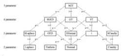
Special and limiting cases of the skewed generalized t distribution include the skewed generalized error distribution, the generalized t distribution introduced by McDonald and Newey,^[6] the skewed t proposed by Hansen,^[8] the skewed Laplace distribution, the generalized error distribution (also known as the generalized normal distribution), a skewed normal distribution, the student t distribution, the skewed Cauchy distribution, the Laplace distribution, the uniform distribution, the normal distribution, and the Cauchy distribution. The graphic below, adapted from Hansen, McDonald, and Newey,^[2] shows which parameters should be set to obtain some of the different special values of the skewed generalized t distribution.

The Skewed Generalized Error Distribution (SGED) has the pdf:

${\displaystyle \lim _{q\to \infty }f_{\text{SGT}}(x;\mu ,\sigma ,\lambda ,p,q)}$

${\displaystyle =f_{\text{SGED}}(x;\mu ,\sigma ,\lambda ,p)={\frac {p}{2v\sigma \Gamma ({\frac {1}{p}})}}e^{-\left({\frac {|x-\mu +m|}{v\sigma [1+\lambda \operatorname {sgn}(x-\mu +m)]}}\right)^{p}}}$

where

${\displaystyle m=\lambda v\sigma {\frac {2^{\frac {2}{p}}\Gamma ({\frac {1}{2}}+{\frac {1}{p}})}{\sqrt {\pi }}}}$

gives a mean of ${\displaystyle \mu }$. Also

${\displaystyle v={\sqrt {\frac {\pi \Gamma ({\frac {1}{p}})}{\pi (1+3\lambda ^{2})\Gamma ({\frac {3}{p}})-16^{\frac {1}{p}}\lambda ^{2}\Gamma ({\frac {1}{2}}+{\frac {1}{p}})^{2}\Gamma ({\frac {1}{p}})}}}}$

gives a variance of ${\displaystyle \sigma ^{2}}$.

The generalized t-distribution (GT) has the pdf:

${\displaystyle f_{\text{SGT}}(x;\mu ,\sigma ,\lambda {=}0,p,q)}$

${\displaystyle =f_{\text{GT}}(x;\mu ,\sigma ,p,q)={\frac {p}{2v\sigma q^{\frac {1}{p}}B({\frac {1}{p}},q)\left[1+{\frac {\left|x-\mu \right|^{p}}{q(v\sigma )^{p}}}\right]^{{\frac {1}{p}}+q}}}}$

where

${\displaystyle v={\frac {1}{q^{\frac {1}{p}}}}{\sqrt {\frac {B({\frac {1}{p}},q)}{B({\frac {3}{p}},q-{\frac {2}{p}})}}}}$

gives a variance of ${\displaystyle \sigma ^{2}}$.

The skewed t-distribution (ST) has the pdf:

${\displaystyle f_{\text{SGT}}(x;\mu ,\sigma ,\lambda ,p{=}2,q)}$

${\displaystyle =f_{\text{ST}}(x;\mu ,\sigma ,\lambda ,q)={\frac {\Gamma ({\frac {1}{2}}+q)}{v\sigma (\pi q)^{\frac {1}{2}}\Gamma (q)\left[1+{\frac {\left|x-\mu +m\right|^{2}}{q(v\sigma )^{2}(1+\lambda \operatorname {sgn}(x-\mu +m))^{2}}}\right]^{{\frac {1}{2}}+q}}}}$

where

${\displaystyle m=\lambda v\sigma {\frac {2q^{\frac {1}{2}}\Gamma (q-{\frac {1}{2}})}{\pi ^{\frac {1}{2}}\Gamma (q)}}}$

gives a mean of ${\displaystyle \mu }$. Also

${\displaystyle v={\frac {1}{q^{\frac {1}{2}}{\sqrt {(1+3\lambda ^{2}){\frac {1}{2q-2}}-{\frac {4\lambda ^{2}}{\pi }}\left({\frac {\Gamma (q-{\frac {1}{2}})}{\Gamma (q)}}\right)^{2}}}}}}$

gives a variance of ${\displaystyle \sigma ^{2}}$.

The skewed Laplace distribution (SLaplace) has the pdf:

${\displaystyle \lim _{q\to \infty }f_{\text{SGT}}(x;\mu ,\sigma ,\lambda ,p{=}1,q)}$

${\displaystyle =f_{\text{SLaplace}}(x;\mu ,\sigma ,\lambda )={\frac {1}{2v\sigma }}e^{-{\frac {|x-\mu +m|}{v\sigma (1+\lambda \operatorname {sgn}(x-\mu +m))}}}}$

where

${\displaystyle m=2v\sigma \lambda }$

gives a mean of ${\displaystyle \mu }$. Also

${\displaystyle v=[2(1+\lambda ^{2})]^{-{\frac {1}{2}}}}$

gives a variance of ${\displaystyle \sigma ^{2}}$.

The generalized error distribution (GED, also known as the generalized normal distribution) has the pdf:

${\displaystyle \lim _{q\to \infty }f_{\text{SGT}}(x;\mu ,\sigma ,\lambda {=}0,p,q)}$

${\displaystyle =f_{\text{GED}}(x;\mu ,\sigma ,p)={\frac {p}{2v\sigma \Gamma ({\frac {1}{p}})}}e^{-\left({\frac {|x-\mu |}{v\sigma }}\right)^{p}}}$

where

${\displaystyle v={\sqrt {\frac {\Gamma ({\frac {1}{p}})}{\Gamma ({\frac {3}{p}})}}}}$

gives a variance of ${\displaystyle \sigma ^{2}}$.

The skewed normal distribution (SNormal) has the pdf:

${\displaystyle \lim _{q\to \infty }f_{\text{SGT}}(x;\mu ,\sigma ,\lambda ,p{=}2,q)}$

${\displaystyle =f_{\text{SNormal}}(x;\mu ,\sigma ,\lambda )={\frac {1}{v\sigma {\sqrt {\pi }}}}e^{-\left[{\frac {|x-\mu +m|}{v\sigma (1+\lambda \operatorname {sgn}(x-\mu +m))}}\right]^{2}}}$

where

${\displaystyle m=\lambda v\sigma {\frac {2}{\sqrt {\pi }}}}$

gives a mean of ${\displaystyle \mu }$. Also

${\displaystyle v={\sqrt {\frac {2\pi }{\pi -8\lambda ^{2}+3\pi \lambda ^{2}}}}}$

gives a variance of ${\displaystyle \sigma ^{2}}$.

The distribution should not be confused with the skew normal distribution or another asymmetric version. Indeed, the distribution here is a special case of a bi-Gaussian, whose left and right widths are proportional to ${\displaystyle 1-\lambda }$ and ${\displaystyle 1+\lambda }$.

The Student's t-distribution (T) has the pdf:

${\displaystyle f_{\text{SGT}}(x;\mu {=}0,\sigma {=}1,\lambda {=}0,p{=}2,q{=}{\tfrac {d}{2}})}$

${\displaystyle =f_{\text{T}}(x;d)={\frac {\Gamma ({\frac {d+1}{2}})}{(\pi d)^{\frac {1}{2}}\Gamma ({\frac {d}{2}})}}\left(1+{\frac {x^{2}}{d}}\right)^{-{\frac {d+1}{2}}}}$

${\displaystyle v={\sqrt {2}}}$ was substituted.

The skewed cauchy distribution (SCauchy) has the pdf:

${\displaystyle f_{\text{SGT}}(x;\mu ,\sigma ,\lambda ,p{=}2,q{=}{\tfrac {1}{2}})}$

${\displaystyle =f_{\text{SCauchy}}(x;\mu ,\sigma ,\lambda )={\frac {1}{\sigma \pi \left[1+{\frac {\left|x-\mu \right|^{2}}{\sigma ^{2}(1+\lambda \operatorname {sgn}(x-\mu ))^{2}}}\right]}}}$

${\displaystyle v={\sqrt {2}}}$ and ${\displaystyle m=0}$ was substituted.

The mean, variance, skewness, and kurtosis of the skewed Cauchy distribution are all undefined.

The Laplace distribution has the pdf:

${\displaystyle \lim _{q\to \infty }f_{\text{SGT}}(x;\mu ,\sigma ,\lambda {=}0,p{=}1,q)}$

${\displaystyle =f_{\text{Laplace}}(x;\mu ,\sigma )={\frac {1}{2\sigma }}e^{-{\frac {|x-\mu |}{\sigma }}}}$

${\displaystyle v=1}$ was substituted.

The uniform distribution has the pdf:

${\displaystyle \lim _{p\to \infty }f_{\text{SGT}}(x;\mu ,\sigma ,\lambda ,p,q)}$

${\displaystyle =f(x)={\begin{cases}{\frac {1}{2v\sigma }}&|x-\mu |<v\sigma \\0&\mathrm {otherwise} \end{cases}}}$

Thus the standard uniform parameterization is obtained if ${\displaystyle \mu ={\frac {a+b}{2}}}$, ${\displaystyle v=1}$, and ${\displaystyle \sigma ={\frac {b-a}{2}}}$.

The normal distribution has the pdf:

${\displaystyle \lim _{q\to \infty }f_{\text{SGT}}(x;\mu ,\sigma ,\lambda {=}0,p{=}2,q)}$

${\displaystyle =f_{\text{Normal}}(x;\mu ,\sigma )={\frac {e^{-\left({\frac {|x-\mu |}{v\sigma }}\right)^{2}}}{v\sigma {\sqrt {\pi }}}}}$

where

${\displaystyle v={\sqrt {2}}}$

gives a variance of ${\displaystyle \sigma ^{2}}$.

The Cauchy distribution has the pdf:

${\displaystyle f_{\text{SGT}}(x;\mu ,\sigma ,\lambda {=}0,p{=}2,q{=}{\tfrac {1}{2}})}$

${\displaystyle =f_{\text{Cauchy}}(x;\mu ,\sigma )={\frac {1}{\sigma \pi \left[1+\left({\frac {x-\mu }{\sigma }}\right)^{2}\right]}}}$

${\displaystyle v={\sqrt {2}}}$ was substituted.

• Hansen, B. (1994). "Autoregressive Conditional Density Estimation". International Economic Review. 35 (3): 705–730. doi:10.2307/2527081. JSTOR 2527081.
• Hansen, C.; McDonald, J.; Newey, W. (2010). "Instrumental Variables Estimation with Flexible Distributions". Journal of Business and Economic Statistics. 28: 13–25. doi:10.1198/jbes.2009.06161. hdl:10419/79273. S2CID 11370711.
• Hansen, C.; McDonald, J.; Theodossiou, P. (2007). "Some Flexible Parametric Models for Partially Adaptive Estimators of Econometric Models". Economics: The Open-Access, Open-Assessment e-Journal. 1 (2007–7): 1. doi:10.5018/economics-ejournal.ja.2007-7. hdl:20.500.14279/1024.
• McDonald, J.; Michefelder, R.; Theodossiou, P. (2009). "Evaluation of Robust Regression Estimation Methods and Intercept Bias: A Capital Asset Pricing Model Application" (PDF). Multinational Finance Journal. 15 (3/4): 293–321. doi:10.17578/13-3/4-6. S2CID 15012865.
• McDonald, J.; Michelfelder, R.; Theodossiou, P. (2010). "Robust Estimation with Flexible Parametric Distributions: Estimation of Utility Stock Betas". Quantitative Finance. 10 (4): 375–387. doi:10.1080/14697680902814241. S2CID 11130911.
• McDonald, J.; Newey, W. (1988). "Partially Adaptive Estimation of Regression Models via the Generalized t Distribution". Econometric Theory. 4 (3): 428–457. doi:10.1017/s0266466600013384. S2CID 120305707.
• Savva, C.; Theodossiou, P. (2015). "Skewness and the Relation between Risk and Return". Management Science.
• Theodossiou, P. (1998). "Financial Data and the Skewed Generalized T Distribution". Management Science. 44 (12–part–1): 1650–1661. doi:10.1287/mnsc.44.12.1650.

• outlines skewed generalized t distribution, its special cases, and a program to calculate its pdf, cdf, and critical values
• online demo https://www.desmos.com/calculator/hfb11etkeq