Rectangular function with a = 1 The rectangular function  (also known as the rectangle function , rect function , Pi function , Heaviside Pi function ,[ 1] gate function , unit pulse , or the normalized boxcar function  ) is defined as[ 2] 


        rect 
         
        
          ( 
          
            
              t 
              a 
             
           
          ) 
         
        = 
        Π 
        
          ( 
          
            
              t 
              a 
             
           
          ) 
         
        = 
        
          { 


                  0 
                  , 


                    if  
                   
                  
                    | 
                   
                  t 
                  
                    | 
                   
                  > 
                  
                    
                      a 
                      2 


                      1 
                      2 
                     
                   
                  , 


                    if  
                   
                  
                    | 
                   
                  t 
                  
                    | 
                   
                  = 
                  
                    
                      a 
                      2 


                  1 
                  , 


                    if  
                   
                  
                    | 
                   
                  t 
                  
                    | 
                   
                  < 
                  
                    
                      a 
                      2 
                     
                   
                  . 


    {\displaystyle \operatorname {rect} \left({\frac {t}{a}}\right)=\Pi \left({\frac {t}{a}}\right)=\left\{{\begin{array}{rl}0,&{\text{if }}|t|>{\frac {a}{2}}\\{\frac {1}{2}},&{\text{if }}|t|={\frac {a}{2}}\\1,&{\text{if }}|t|<{\frac {a}{2}}.\end{array}}\right.} 
   
 
Alternative definitions of the function define 


        rect 
         
        
          ( 
          
            ± 
            
              
                1 
                2 


          ) 


    {\textstyle \operatorname {rect} \left(\pm {\frac {1}{2}}\right)} 
   
 [ 3] [ 4] [ 5] 
Its periodic version is called a rectangular wave 
History 
The rect  function has been introduced 1953 by Woodward [ 6] [ 7] cutout operator , together with the sinc  function[ 8] [ 9] interpolation operator , and their counter operations which are sampling  (comb  operatorreplicating  (rep  operator
Relation to the boxcar function 
The rectangular function is a special case of the more general boxcar function :


        rect 
         
        
          ( 


                t 
                − 
                X 
               
              Y 
             
           
          ) 
         
        = 
        H 
        ( 
        t 
        − 
        ( 
        X 
        − 
        Y 
        
          / 
         
        2 
        ) 
        ) 
        − 
        H 
        ( 
        t 
        − 
        ( 
        X 
        + 
        Y 
        
          / 
         
        2 
        ) 
        ) 
        = 
        H 
        ( 
        t 
        − 
        X 
        + 
        Y 
        
          / 
         
        2 
        ) 
        − 
        H 
        ( 
        t 
        − 
        X 
        − 
        Y 
        
          / 
         
        2 
        ) 
       
     
    {\displaystyle \operatorname {rect} \left({\frac {t-X}{Y}}\right)=H(t-(X-Y/2))-H(t-(X+Y/2))=H(t-X+Y/2)-H(t-X-Y/2)} 
   
 
where 


        H 
        ( 
        x 
        ) 
       
     
    {\displaystyle H(x)} 
   
 Heaviside step function ; the function is centered at 


        X 
       
     
    {\displaystyle X} 


        Y 
       
     
    {\displaystyle Y} 


        X 
        − 
        Y 
        
          / 
         
        2 
       
     
    {\displaystyle X-Y/2} 


        X 
        + 
        Y 
        
          / 
         
        2. 
       
     
    {\displaystyle X+Y/2.} 
   
 
Plot of normalized 


        sinc 
         
        ( 
        x 
        ) 
       
     
    {\displaystyle \operatorname {sinc} (x)} 


        sinc 
         
        ( 
        π 
        x 
        ) 
       
     
    {\displaystyle \operatorname {sinc} (\pi x)} 
   
  The unitary Fourier transforms  of the rectangular function are[ 2] 


          ∫ 
          
            − 
            ∞ 
           
          
            ∞ 
           
         
        rect 
         
        ( 
        t 
        ) 
        ⋅ 
        
          e 
          
            − 
            i 
            2 
            π 
            f 
            t 
           
         
        d 
        t 
        = 


              sin 
               
              ( 
              π 
              f 
              ) 
             
            
              π 
              f 


        = 
        sinc 
         
        ( 
        π 
        f 
        ) 
        = 
        
          sinc 
          
            π 


        ( 
        f 
        ) 
        , 
       
     
    {\displaystyle \int _{-\infty }^{\infty }\operatorname {rect} (t)\cdot e^{-i2\pi ft}\,dt={\frac {\sin(\pi f)}{\pi f}}=\operatorname {sinc} (\pi f)=\operatorname {sinc} _{\pi }(f),} 
   
 f , where 


          sinc 
          
            π 


    {\displaystyle \operatorname {sinc} _{\pi }} 
   
 [ 10] sinc function  and


            1 
            
              2 
              π 


          ∫ 
          
            − 
            ∞ 
           
          
            ∞ 
           
         
        rect 
         
        ( 
        t 
        ) 
        ⋅ 
        
          e 
          
            − 
            i 
            ω 
            t 
           
         
        d 
        t 
        = 
        
          
            1 
            
              2 
              π 


        ⋅ 


              sin 
               
              
                ( 
                
                  ω 
                  
                    / 
                   
                  2 
                 
                ) 


              ω 
              
                / 
               
              2 


        = 
        
          
            1 
            
              2 
              π 


        ⋅ 
        sinc 
         
        
          ( 
          
            ω 
            
              / 
             
            2 
           
          ) 
         
        , 
       
     
    {\displaystyle {\frac {1}{\sqrt {2\pi }}}\int _{-\infty }^{\infty }\operatorname {rect} (t)\cdot e^{-i\omega t}\,dt={\frac {1}{\sqrt {2\pi }}}\cdot {\frac {\sin \left(\omega /2\right)}{\omega /2}}={\frac {1}{\sqrt {2\pi }}}\cdot \operatorname {sinc} \left(\omega /2\right),} 


        ω 
       
     
    {\displaystyle \omega } 


        sinc 
       
     
    {\displaystyle \operatorname {sinc} } 
   
 sinc function .
For 


        rect 
         
        ( 
        x 
        
          / 
         
        a 
        ) 
       
     
    {\displaystyle \operatorname {rect} (x/a)} 


          ∫ 
          
            − 
            ∞ 
           
          
            ∞ 
           
         
        rect 
         
        
          ( 
          
            
              t 
              a 
             
           
          ) 
         
        ⋅ 
        
          e 
          
            − 
            i 
            2 
            π 
            f 
            t 
           
         
        d 
        t 
        = 
        a 


              sin 
               
              ( 
              π 
              a 
              f 
              ) 
             
            
              π 
              a 
              f 


        = 
        a 
          
        
          sinc 
          
            π 


          ( 
          a 
          f 
          ) 
         
        . 
       
     
    {\displaystyle \int _{-\infty }^{\infty }\operatorname {rect} \left({\frac {t}{a}}\right)\cdot e^{-i2\pi ft}\,dt=a{\frac {\sin(\pi af)}{\pi af}}=a\ \operatorname {sinc} _{\pi }{(af)}.} 
   
 
Relation to the triangular function 
We can define the triangular function  as the convolution  of two rectangular functions:


          t 
          r 
          i 
          ( 
          t 
          
            / 
           
          T 
          ) 
         
        = 
        
          r 
          e 
          c 
          t 
          ( 
          2 
          t 
          
            / 
           
          T 
          ) 
         
        ∗ 
        
          r 
          e 
          c 
          t 
          ( 
          2 
          t 
          
            / 
           
          T 
          ) 
         
        . 
         
     
    {\displaystyle \operatorname {tri(t/T)} =\operatorname {rect(2t/T)} *\operatorname {rect(2t/T)} .\,} 
   
 
Use in probability 
Viewing the rectangular function as a probability density function , it is a special case of the continuous uniform distribution  with 


        a 
        = 
        − 
        1 
        
          / 
         
        2 
        , 
        b 
        = 
        1 
        
          / 
         
        2. 
       
     
    {\displaystyle a=-1/2,b=1/2.} 
   
 characteristic function  is


        φ 
        ( 
        k 
        ) 
        = 


              sin 
               
              ( 
              k 
              
                / 
               
              2 
              ) 
             
            
              k 
              
                / 
               
              2 


        , 
       
     
    {\displaystyle \varphi (k)={\frac {\sin(k/2)}{k/2}},} 
   
 
and its moment-generating function  is


        M 
        ( 
        k 
        ) 
        = 


              sinh 
               
              ( 
              k 
              
                / 
               
              2 
              ) 
             
            
              k 
              
                / 
               
              2 


        , 
       
     
    {\displaystyle M(k)={\frac {\sinh(k/2)}{k/2}},} 
   
 
where 


        sinh 
         
        ( 
        t 
        ) 
       
     
    {\displaystyle \sinh(t)} 
   
 hyperbolic sine  function.
Rational approximation 
The pulse function may also be expressed as a limit of a rational function :


        Π 
        ( 
        t 
        ) 
        = 
        
          lim 
          
            n 
            → 
            ∞ 
            , 
            n 
            ∈ 
            
              ( 
             
            Z 
            ) 


            1 
            
              ( 
              2 
              t 
              
                ) 
                
                  2 
                  n 
                 
               
              + 
              1 


        . 
       
     
    {\displaystyle \Pi (t)=\lim _{n\rightarrow \infty ,n\in \mathbb {(} Z)}{\frac {1}{(2t)^{2n}+1}}.} 
   
 
Demonstration of validity 
First, we consider the case where 


          | 
         
        t 
        
          | 
         
        < 
        
          
            1 
            2 
           
         
        . 
       
     
    {\textstyle |t|<{\frac {1}{2}}.} 


        ( 
        2 
        t 
        
          ) 
          
            2 
            n 


    {\textstyle (2t)^{2n}} 


        n 
        . 
       
     
    {\displaystyle n.} 


        2 
        t 
        < 
        1 
       
     
    {\displaystyle 2t<1} 


        ( 
        2 
        t 
        
          ) 
          
            2 
            n 


    {\textstyle (2t)^{2n}} 


        n 
        . 
       
     
    {\displaystyle n.} 
   
 
It follows that:


          lim 
          
            n 
            → 
            ∞ 
            , 
            n 
            ∈ 
            
              ( 
             
            Z 
            ) 


            1 
            
              ( 
              2 
              t 
              
                ) 
                
                  2 
                  n 
                 
               
              + 
              1 


        = 
        
          
            1 
            
              0 
              + 
              1 


        = 
        1 
        , 
        
          | 
         
        t 
        
          | 
         
        < 


              1 
              2 


        . 
       
     
    {\displaystyle \lim _{n\rightarrow \infty ,n\in \mathbb {(} Z)}{\frac {1}{(2t)^{2n}+1}}={\frac {1}{0+1}}=1,|t|<{\tfrac {1}{2}}.} 
   
 
Second, we consider the case where 


          | 
         
        t 
        
          | 
         
        > 
        
          
            1 
            2 
           
         
        . 
       
     
    {\textstyle |t|>{\frac {1}{2}}.} 


        ( 
        2 
        t 
        
          ) 
          
            2 
            n 


    {\textstyle (2t)^{2n}} 


        n 
        . 
       
     
    {\displaystyle n.} 


        2 
        t 
        > 
        1 
       
     
    {\displaystyle 2t>1} 


        ( 
        2 
        t 
        
          ) 
          
            2 
            n 


    {\textstyle (2t)^{2n}} 


        n 
        . 
       
     
    {\displaystyle n.} 
   
 
It follows that:


          lim 
          
            n 
            → 
            ∞ 
            , 
            n 
            ∈ 
            
              ( 
             
            Z 
            ) 


            1 
            
              ( 
              2 
              t 
              
                ) 
                
                  2 
                  n 
                 
               
              + 
              1 


        = 
        
          
            1 
            
              + 
              ∞ 
              + 
              1 


        = 
        0 
        , 
        
          | 
         
        t 
        
          | 
         
        > 


              1 
              2 


        . 
       
     
    {\displaystyle \lim _{n\rightarrow \infty ,n\in \mathbb {(} Z)}{\frac {1}{(2t)^{2n}+1}}={\frac {1}{+\infty +1}}=0,|t|>{\tfrac {1}{2}}.} 
   
 
Third, we consider the case where 


          | 
         
        t 
        
          | 
         
        = 
        
          
            1 
            2 
           
         
        . 
       
     
    {\textstyle |t|={\frac {1}{2}}.} 


          lim 
          
            n 
            → 
            ∞ 
            , 
            n 
            ∈ 
            
              ( 
             
            Z 
            ) 


            1 
            
              ( 
              2 
              t 
              
                ) 
                
                  2 
                  n 
                 
               
              + 
              1 


        = 
        
          lim 
          
            n 
            → 
            ∞ 
            , 
            n 
            ∈ 
            
              ( 
             
            Z 
            ) 


            1 
            
              
                1 
                
                  2 
                  n 
                 
               
              + 
              1 


        = 
        
          
            1 
            
              1 
              + 
              1 


        = 


              1 
              2 


        . 
       
     
    {\displaystyle \lim _{n\rightarrow \infty ,n\in \mathbb {(} Z)}{\frac {1}{(2t)^{2n}+1}}=\lim _{n\rightarrow \infty ,n\in \mathbb {(} Z)}{\frac {1}{1^{2n}+1}}={\frac {1}{1+1}}={\tfrac {1}{2}}.} 
   
 
We see that it satisfies the definition of the pulse function. Therefore,


        rect 
         
        ( 
        t 
        ) 
        = 
        Π 
        ( 
        t 
        ) 
        = 
        
          lim 
          
            n 
            → 
            ∞ 
            , 
            n 
            ∈ 
            
              ( 
             
            Z 
            ) 


            1 
            
              ( 
              2 
              t 
              
                ) 
                
                  2 
                  n 
                 
               
              + 
              1 


        = 
        
          
            { 


                  0 


                      if  


                    | 
                   
                  t 
                  
                    | 
                   
                  > 
                  
                    
                      1 
                      2 


                      1 
                      2 


                      if  


                    | 
                   
                  t 
                  
                    | 
                   
                  = 
                  
                    
                      1 
                      2 


                  1 


                      if  


                    | 
                   
                  t 
                  
                    | 
                   
                  < 
                  
                    
                      1 
                      2 
                     
                   
                  . 


    {\displaystyle \operatorname {rect} (t)=\Pi (t)=\lim _{n\rightarrow \infty ,n\in \mathbb {(} Z)}{\frac {1}{(2t)^{2n}+1}}={\begin{cases}0&{\mbox{if }}|t|>{\frac {1}{2}}\\{\frac {1}{2}}&{\mbox{if }}|t|={\frac {1}{2}}\\1&{\mbox{if }}|t|<{\frac {1}{2}}.\\\end{cases}}} 
   
 
Dirac delta function 
The rectangle function can be used to represent the Dirac delta function  


        δ 
        ( 
        x 
        ) 
       
     
    {\displaystyle \delta (x)} 
   
 [ 11] 


        δ 
        ( 
        x 
        ) 
        = 
        
          lim 
          
            a 
            → 
            0 


            1 
            a 
           
         
        rect 
         
        
          ( 
          
            
              x 
              a 
             
           
          ) 
         
        . 
       
     
    {\displaystyle \delta (x)=\lim _{a\to 0}{\frac {1}{a}}\operatorname {rect} \left({\frac {x}{a}}\right).} 


        g 
        ( 
        x 
        ) 
       
     
    {\displaystyle g(x)} 


        a 
       
     
    {\displaystyle a} 


          g 
          
            a 
            v 
            g 
           
         
        ( 
        0 
        ) 
        = 
        
          
            1 
            a 


          ∫ 
          
            − 
            ∞ 
           
          
            ∞ 
           
         
        d 
        x 
          
        g 
        ( 
        x 
        ) 
        rect 
         
        
          ( 
          
            
              x 
              a 
             
           
          ) 
         
        . 
       
     
    {\displaystyle g_{avg}(0)={\frac {1}{a}}\int \limits _{-\infty }^{\infty }dx\ g(x)\operatorname {rect} \left({\frac {x}{a}}\right).} 


        g 
        ( 
        0 
        ) 
       
     
    {\displaystyle g(0)} 


        g 
        ( 
        0 
        ) 
        = 
        
          lim 
          
            a 
            → 
            0 


            1 
            a 


          ∫ 
          
            − 
            ∞ 
           
          
            ∞ 
           
         
        d 
        x 
          
        g 
        ( 
        x 
        ) 
        rect 
         
        
          ( 
          
            
              x 
              a 
             
           
          ) 


    {\displaystyle g(0)=\lim _{a\to 0}{\frac {1}{a}}\int \limits _{-\infty }^{\infty }dx\ g(x)\operatorname {rect} \left({\frac {x}{a}}\right)} 


        g 
        ( 
        0 
        ) 
        = 
        
          ∫ 
          
            − 
            ∞ 
           
          
            ∞ 
           
         
        d 
        x 
          
        g 
        ( 
        x 
        ) 
        δ 
        ( 
        x 
        ) 
        . 
       
     
    {\displaystyle g(0)=\int \limits _{-\infty }^{\infty }dx\ g(x)\delta (x).} 


        δ 
        ( 
        t 
        ) 
       
     
    {\displaystyle \delta (t)} 


        δ 
        ( 
        f 
        ) 
        = 
        
          ∫ 
          
            − 
            ∞ 
           
          
            ∞ 
           
         
        δ 
        ( 
        t 
        ) 
        ⋅ 
        
          e 
          
            − 
            i 
            2 
            π 
            f 
            t 
           
         
        d 
        t 
        = 
        
          lim 
          
            a 
            → 
            0 


            1 
            a 


          ∫ 
          
            − 
            ∞ 
           
          
            ∞ 
           
         
        rect 
         
        
          ( 
          
            
              t 
              a 
             
           
          ) 
         
        ⋅ 
        
          e 
          
            − 
            i 
            2 
            π 
            f 
            t 
           
         
        d 
        t 
        = 
        
          lim 
          
            a 
            → 
            0 
           
         
        sinc 
         
        
          ( 
          a 
          f 
          ) 
         
        . 
       
     
    {\displaystyle \delta (f)=\int _{-\infty }^{\infty }\delta (t)\cdot e^{-i2\pi ft}\,dt=\lim _{a\to 0}{\frac {1}{a}}\int _{-\infty }^{\infty }\operatorname {rect} \left({\frac {t}{a}}\right)\cdot e^{-i2\pi ft}\,dt=\lim _{a\to 0}\operatorname {sinc} {(af)}.} 
   
 sinc function  here is the normalized sinc function. Because the first zero of the sinc function is at 


        f 
        = 
        1 
        
          / 
         
        a 
       
     
    {\displaystyle f=1/a} 


        a 
       
     
    {\displaystyle a} 


        δ 
        ( 
        t 
        ) 
       
     
    {\displaystyle \delta (t)} 


        δ 
        ( 
        f 
        ) 
        = 
        1 
        , 
       
     
    {\displaystyle \delta (f)=1,} 
   
 
See also 
References 
^ Wolfram Research (2008). "HeavisidePi, Wolfram Language function" . Retrieved October 11,  2022 . ^ a b   Weisstein, Eric W.  "Rectangle Function" . MathWorld ^ Wang, Ruye (2012). Introduction to Orthogonal Transforms: With Applications in Data Processing and Analysis 135– 136. ISBN  9780521516884 . ^ Tang, K. T. (2007). Mathematical Methods for Engineers and Scientists: Fourier analysis, partial differential equations and variational models ISBN  9783540446958 . ^ Kumar, A. Anand (2011). Signals and Systems 258– 260. ISBN  9788120343108 . ^ Klauder, John R (1960). "The Theory and Design of Chirp Radars" Bell System Technical Journal . 39  (4): 745– 808. doi :10.1002/j.1538-7305.1960.tb03942.x . ^ Woodward, Philipp M (1953). Probability and Information Theory, with Applications to Radar . Pergamon Press. p. 29. ^ Higgins, John Rowland (1996). Sampling Theory in Fourier and Signal Analysis: Foundations . Oxford University Press Inc. p. 4. ISBN  0198596995 . ^ Zayed, Ahmed I (1996). Handbook of Function and Generalized Function Transformations . CRC Press. p. 507. ISBN  9780849380761 . ^ Wolfram MathWorld, https://mathworld.wolfram.com/SincFunction.html  
^ Khare, Kedar; Butola, Mansi; Rajora, Sunaina (2023). "Chapter 2.4 Sampling by Averaging, Distributions and Delta Function". Fourier Optics and Computational Imaging  (2nd ed.). Springer. pp. 15– 16. doi :10.1007/978-3-031-18353-9 . ISBN  978-3-031-18353-9 .
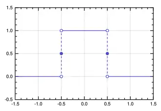