Seiberg–Witten flow

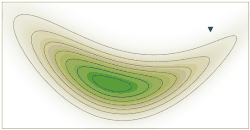
In differential geometry, the Seiberg–Witten flow is a gradient flow described by the Seiberg–Witten equations, hence a method to describe a gradient descent of the Seiberg–Witten action functional. Simply put, the Seiberg–Witten flow is a path always going in the direction of steepest descent, similar to the path of a ball rolling down a hill. This helps to find critical points, called (Seiberg–Witten) monopoles, which solve the Seiberg–Witten equations. Illustratively, they are the points on the hill on which the ball can rest.

The Seiberg–Witten flow is named after Nathan Seiberg and Edward Witten, who first formulated the underlying Seiberg–Witten theory in 1994.

Let ${\displaystyle M}$ be a compact orientable Riemannian 4-manifold. Every such manifold has a spin^c structure,^[1] which is a lift of the classifying map ${\displaystyle f\colon M\rightarrow \operatorname {BSO} (4)}$ of the tangent bundle ${\displaystyle TM}$ (hence so that ${\displaystyle TM\cong f^{*}{\widetilde {\gamma }}_{\mathbb {R} }^{4}}$ is the pullback bundle of the oriented tautological bundle along it) to a continuous map ${\displaystyle {\widehat {f}}\colon M\rightarrow \operatorname {BSpin} ^{\mathrm {c} }(4)}$ (hence so that it factors over the map induced by the canonical projection ${\displaystyle \operatorname {Spin} ^{\mathrm {c} }(4)\twoheadrightarrow \operatorname {SO} (4)}$ on classifying spaces). All possible spin^c structures correspond exactly to the second singular cohomology ${\displaystyle H^{2}(M,\mathbb {Z} )\cong [M,\operatorname {BU} (1)]}$. Because of the central identity:

${\displaystyle \operatorname {Spin} ^{\mathrm {c} }(4)\cong \operatorname {U} (2)\times _{\operatorname {U} (1)}\operatorname {U} (2)\cong \left\{A^{\pm }\in \operatorname {U} (2)|\det(A^{-})=\det(A^{+})\right\},}$

the spin^c structure classifies complex plane bundles ${\displaystyle S^{\pm }\twoheadrightarrow M}$ with same determinant line bundle ${\displaystyle L=\det(S^{\pm })}$. Over the frame bundle, it corresponds to a principal U(1)-bundle ${\displaystyle \operatorname {Fr} _{\operatorname {U} }(L)\twoheadrightarrow M}$, which fulfills ${\displaystyle L\cong \operatorname {Fr} _{\operatorname {U} }(L)\times _{\operatorname {U} (1)}\mathbb {C} }$ using the balanced product and with trivial adjoint bundle ${\displaystyle \operatorname {Ad} \operatorname {Fr} _{\operatorname {U} }(L)\cong {\underline {\operatorname {End} }}(L)\cong {\underline {\mathbb {C} }}}$. Furthermore let ${\displaystyle S=S^{-}\oplus S^{+}}$ with the Whitney sum. Since the determinant line bundle preserves the first Chern class, which also describes the isomorphism required between cohomology and homotopy classes here, one has ${\displaystyle c_{1}(L)=c_{1}(S^{\pm })\in H^{2}(M,\mathbb {Z} )\cong [M,\operatorname {BU} (1)]}$, which is additionally the same class as for the spin^c structure. For a connection ${\displaystyle A\in \Omega _{\operatorname {Ad} }^{1}(\operatorname {Fr} _{\operatorname {U} }(L),{\mathfrak {u}}(1))\cong \Omega ^{1}(B)}$ with curvature form ${\displaystyle F_{A}=\mathrm {d} A}$, it can also be calculated using Chern–Weil theory:

${\displaystyle -8\pi ^{2}c_{1}(L)=\int _{B}\operatorname {tr} (F_{A}\wedge F_{A})\mathrm {d} \operatorname {vol} _{g}=\int _{B}|F_{A}^{+}|^{2}-|F_{A}^{-}|^{2}\mathrm {d} \operatorname {vol} _{g}.}$

The Seiberg–Witten action functional is given by:^[2][3]

${\displaystyle \operatorname {SW} \colon \Omega ^{1}(M,\operatorname {Ad} (L))\times \Gamma ^{\infty }(M,S^{+})\rightarrow \mathbb {R} ,\operatorname {SW} (A,\Phi ):=\int _{B}{\frac {1}{2}}\|F_{A}^{+}\|^{2}+\|\nabla _{A}\Phi \|^{2}+{\frac {\operatorname {scal} }{4}}\|\Phi \|^{2}+{\frac {1}{8}}\|\Phi \|^{4}\mathrm {d} \operatorname {vol} _{g}.}$

with ${\displaystyle \operatorname {scal} }$ denoting scalar curvature. Using the following relation from Chern–Weil theory:

${\displaystyle \|F_{A}^{+}\|_{L^{2}}=2\|F_{A}\|_{L^{2}}-4\pi ^{2}c_{1}(L)^{2},}$

it can also be rewritten as:

${\displaystyle \operatorname {SW} (A,\Phi ):=\int _{B}\|F_{A}\|^{2}+\|\nabla _{A}\Phi \|^{2}+{\frac {\operatorname {scal} }{4}}\|\Phi \|^{2}+{\frac {1}{8}}\|\Phi \|^{4}\mathrm {d} \operatorname {vol} _{g}+\pi ^{2}c_{1}(L)^{2},}$

but the last term is constant and can be obmitted. Its first two terms are also called Yang–Mills–Higgs action and its first term is also called Yang–Mills action.

Hence the gradient of the Seiberg–Witten action functional gives exactly the Seiberg–Witten equations:

${\displaystyle \operatorname {grad} (\operatorname {SW} )(A,\Phi )_{1}=\mathrm {d} ^{*}F_{A}+i\operatorname {Im} \langle \nabla _{A}\Phi ,\Phi \rangle ,}$

${\displaystyle \operatorname {grad} (\operatorname {SW} )(A,\Phi )_{2}=\nabla _{A}^{*}\nabla _{A}\Phi -{\frac {1}{4}}(\operatorname {scal} +\|\Phi \|^{2})\Phi .}$

For an open interval ${\displaystyle I\subseteq \mathbb {R} }$, two ${\displaystyle C^{1}}$ maps ${\displaystyle \alpha \colon I\rightarrow \Omega ^{1}(M,\operatorname {Ad} (L))}$ and ${\displaystyle \varphi \colon I\rightarrow \Gamma ^{\infty }(M,S^{+})}$ (hence continuously differentiable) fulfilling:

${\displaystyle \alpha '(t)=-\operatorname {grad} (\operatorname {SW} )(\alpha (t),\varphi (t))_{1}=-\mathrm {d} ^{*}F_{\alpha (t)}-i\operatorname {Im} \langle \nabla _{\alpha (t)}\varphi (t),\varphi (t)\rangle }$

${\displaystyle \varphi '(t)=-\operatorname {grad} (\operatorname {SW} )(\alpha (t),\varphi (t))_{2}=-\nabla _{\alpha (t)}^{*}\nabla _{\alpha (t)}\varphi (t)-{\frac {1}{4}}(\operatorname {scal} +\|\varphi (t)\|^{2})\varphi (t)}$

are a Seiberg–Witten flow.^[4][5]

• Liviu I. Nicolaescu, Notes on Seiberg-Witten Theory (PDF)
• Hong, Min-Chun Hong; Schabrun, Lorenz (2009-09-10). "Global Existence for the Seiberg-Witten Flow". arXiv:0909.1855 [math.DG].
• Schabrun, Lorenz (2010-03-09). "Seiberg-Witten Flow in Higher Dimensions". arXiv:1003.1765 [math.DG].

• Yang–Mills flow
• Yang–Mills–Higgs flow

• Seiberg-Witten flow at the nLab

References

^ Nicolaescu, Example 1.3.16
^ Hong & Schabrun 2009, Eq. (4)
^ Schabrun 2010, Eq. (2) & (4)
^ Hong & Schabrun 2009, Eq. (9) & (10)
^ Schabrun 2010, Eq. (7) & (8)