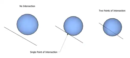
The three possible line-sphere intersections: In analytic geometry , a line  and a sphere  can intersect  in three ways:
No intersection at all 
Intersection in exactly one point 
Intersection in two points. Methods for distinguishing these cases, and determining the coordinates  for the points in the latter cases, are useful in a number of circumstances. For example, it is a common calculation to perform during ray tracing .[ 1] 
Calculation using vectors in 3D 
In vector notation , the equations are as follows:
Equation for a sphere 


            ‖ 
            
              
                x 
               
              − 
              
                c 
               
             
            ‖ 
           
          
            2 
           
         
        = 
        
          r 
          
            2 


    {\displaystyle \left\Vert \mathbf {x} -\mathbf {c} \right\Vert ^{2}=r^{2}} 


          x 


    {\displaystyle \mathbf {x} } 


          c 


    {\displaystyle \mathbf {c} } 


        r 
       
     
    {\displaystyle r} 
   
 Equation for a line starting at 


          o 


    {\displaystyle \mathbf {o} } 


          x 
         
        = 
        
          o 
         
        + 
        d 
        
          u 


    {\displaystyle \mathbf {x} =\mathbf {o} +d\mathbf {u} } 


          x 


    {\displaystyle \mathbf {x} } 


          o 


    {\displaystyle \mathbf {o} } 


        d 
       
     
    {\displaystyle d} 


          u 


    {\displaystyle \mathbf {u} } 
   
 Searching for points that are on the line and on the sphere means combining the equations and solving for 


        d 
       
     
    {\displaystyle d} 
   
 dot product  of vectors:
Equations combined


            ‖ 
            
              
                o 
               
              + 
              d 
              
                u 
               
              − 
              
                c 
               
             
            ‖ 
           
          
            2 
           
         
        = 
        
          r 
          
            2 
           
         
        ⇔ 
        ( 
        
          o 
         
        + 
        d 
        
          u 
         
        − 
        
          c 
         
        ) 
        ⋅ 
        ( 
        
          o 
         
        + 
        d 
        
          u 
         
        − 
        
          c 
         
        ) 
        = 
        
          r 
          
            2 


    {\displaystyle \left\Vert \mathbf {o} +d\mathbf {u} -\mathbf {c} \right\Vert ^{2}=r^{2}\Leftrightarrow (\mathbf {o} +d\mathbf {u} -\mathbf {c} )\cdot (\mathbf {o} +d\mathbf {u} -\mathbf {c} )=r^{2}} 
   
  
Expanded and rearranged:


          d 
          
            2 
           
         
        ( 
        
          u 
         
        ⋅ 
        
          u 
         
        ) 
        + 
        2 
        d 
        [ 
        
          u 
         
        ⋅ 
        ( 
        
          o 
         
        − 
        
          c 
         
        ) 
        ] 
        + 
        ( 
        
          o 
         
        − 
        
          c 
         
        ) 
        ⋅ 
        ( 
        
          o 
         
        − 
        
          c 
         
        ) 
        − 
        
          r 
          
            2 
           
         
        = 
        0 
       
     
    {\displaystyle d^{2}(\mathbf {u} \cdot \mathbf {u} )+2d[\mathbf {u} \cdot (\mathbf {o} -\mathbf {c} )]+(\mathbf {o} -\mathbf {c} )\cdot (\mathbf {o} -\mathbf {c} )-r^{2}=0} 
   
  
The form of a quadratic formula  is now observable. (This quadratic equation is an instance of Joachimsthal's equation.[ 2] 


        a 
        
          d 
          
            2 
           
         
        + 
        b 
        d 
        + 
        c 
        = 
        0 
       
     
    {\displaystyle ad^{2}+bd+c=0} 
   
  
where


        a 
        = 
        
          u 
         
        ⋅ 
        
          u 
         
        = 
        
          
            ‖ 
            
              u 
             
            ‖ 
           
          
            2 


    {\displaystyle a=\mathbf {u} \cdot \mathbf {u} =\left\Vert \mathbf {u} \right\Vert ^{2}} 


        b 
        = 
        2 
        [ 
        
          u 
         
        ⋅ 
        ( 
        
          o 
         
        − 
        
          c 
         
        ) 
        ] 
       
     
    {\displaystyle b=2[\mathbf {u} \cdot (\mathbf {o} -\mathbf {c} )]} 


        c 
        = 
        ( 
        
          o 
         
        − 
        
          c 
         
        ) 
        ⋅ 
        ( 
        
          o 
         
        − 
        
          c 
         
        ) 
        − 
        
          r 
          
            2 
           
         
        = 
        
          
            ‖ 
            
              
                o 
               
              − 
              
                c 
               
             
            ‖ 
           
          
            2 
           
         
        − 
        
          r 
          
            2 


    {\displaystyle c=(\mathbf {o} -\mathbf {c} )\cdot (\mathbf {o} -\mathbf {c} )-r^{2}=\left\Vert \mathbf {o} -\mathbf {c} \right\Vert ^{2}-r^{2}} 
   
  
Simplified


        d 
        = 


              − 
              2 
              [ 
              
                u 
               
              ⋅ 
              ( 
              
                o 
               
              − 
              
                c 
               
              ) 
              ] 
              ± 
              
                
                  ( 
                  2 
                  [ 
                  
                    u 
                   
                  ⋅ 
                  ( 
                  
                    o 
                   
                  − 
                  
                    c 
                   
                  ) 
                  ] 
                  
                    ) 
                    
                      2 
                     
                   
                  − 
                  4 
                  
                    
                      ‖ 
                      
                        u 
                       
                      ‖ 
                     
                    
                      2 
                     
                   
                  ( 
                  
                    
                      ‖ 
                      
                        
                          o 
                         
                        − 
                        
                          c 
                         
                       
                      ‖ 
                     
                    
                      2 
                     
                   
                  − 
                  
                    r 
                    
                      2 
                     
                   
                  ) 


              2 
              
                
                  ‖ 
                  
                    u 
                   
                  ‖ 
                 
                
                  2 


    {\displaystyle d={\frac {-2[\mathbf {u} \cdot (\mathbf {o} -\mathbf {c} )]\pm {\sqrt {(2[\mathbf {u} \cdot (\mathbf {o} -\mathbf {c} )])^{2}-4\left\Vert \mathbf {u} \right\Vert ^{2}(\left\Vert \mathbf {o} -\mathbf {c} \right\Vert ^{2}-r^{2})}}}{2\left\Vert \mathbf {u} \right\Vert ^{2}}}} 
   
  
Note that in the specific case where 


          u 


    {\displaystyle \mathbf {u} } 


            ‖ 
            
              u 
             
            ‖ 
           
          
            2 
           
         
        = 
        1 
       
     
    {\displaystyle \left\Vert \mathbf {u} \right\Vert ^{2}=1} 


                u 
               
              ^ 


    {\displaystyle {\hat {\mathbf {u} }}} 


          u 


    {\displaystyle \mathbf {u} } 


        ∇ 
        = 
        [ 


                u 
               
              ^ 


        ⋅ 
        ( 
        
          o 
         
        − 
        
          c 
         
        ) 
        
          ] 
          
            2 
           
         
        − 
        ( 
        
          
            ‖ 
            
              
                o 
               
              − 
              
                c 
               
             
            ‖ 
           
          
            2 
           
         
        − 
        
          r 
          
            2 
           
         
        ) 
       
     
    {\displaystyle \nabla =[{\hat {\mathbf {u} }}\cdot (\mathbf {o} -\mathbf {c} )]^{2}-(\left\Vert \mathbf {o} -\mathbf {c} \right\Vert ^{2}-r^{2})} 


        d 
        = 
        − 
        [ 


                u 
               
              ^ 


        ⋅ 
        ( 
        
          o 
         
        − 
        
          c 
         
        ) 
        ] 
        ± 
        
          
            ∇ 


    {\displaystyle d=-[{\hat {\mathbf {u} }}\cdot (\mathbf {o} -\mathbf {c} )]\pm {\sqrt {\nabla }}} 
   
  If 


        ∇ 
        < 
        0 
       
     
    {\displaystyle \nabla <0} 
   
  
If 


        ∇ 
        = 
        0 
       
     
    {\displaystyle \nabla =0} 
   
  
If 


        ∇ 
        > 
        0 
       
     
    {\displaystyle \nabla >0} 
   
  
See also 
References 
^ Eberly, David H. (2006). 3D game engine design: a practical approach to real-time computer graphics, 2nd edition . Morgan Kaufmann. p. 698. ISBN  0-12-229063-1 . ^ "Joachimsthal's Equation" .